The X-RISK-CC WebGIS is an interactive platform providing access to consistent information about current and future weather extremes in the Alpine region. Data for 20 climate extreme indices can be displayed through different visualization options.

In the following the contents and main functionalities of the X-RISK-CC WebGIS are described.

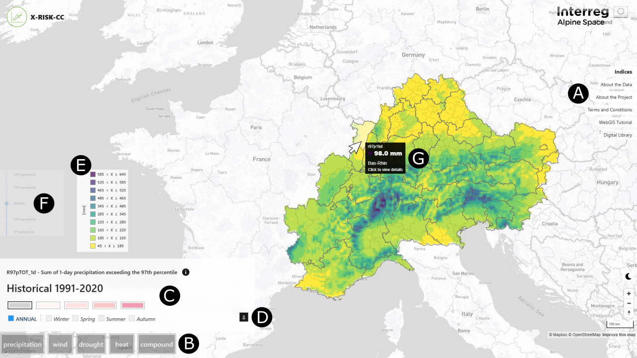
A. List of available resources and documentation:

• Indices: interactive WebGIS section providing index visualization and data download
• About the Data: data sources and citations and technical details about data collection and processing
• About the Project: brief description of the X-RISK-CC project, role of the WebGIS and project partnership
• Terms and Conditions: notes on the WebGIS usage including privacy and data license
• WebGIS Tutorial: details on WebGIS contents and functionalities (this document)
• Digital Library: the digital archive of additional documents complementing the information provided by the WebGIS. It includes scientific reports on weather extreme analysis for the Alpine region and specific study areas, the detailed description of climate indices with recommendations and references, a glossary.

B. Index selection grouped by categories. By moving the cursor over the categories, the list of available indices, reported through their abbreviations, is displayed. By selecting one box, the corresponding index is loaded on the map.

C. The box reports the abbreviation and extended name of the selected index displayed on the map. The "info" button provides further details on the index definition. The index values for the reference period (1991-2020) are visualized by selecting the grey horizontal bar, while the following bars enable the visualization of the projected changes for four increasing Global Warming Levels. The user can select to display the climate index aggregated on an annual or seasonal level. Seasons are defined as follows: December to February for winter, March to May for spring, June to August for summer, September to November for autumn. Note that only projected changes with respect to the reference period are available for GWL layers.

D. Button for data download: the current displayed map can be downloaded as image (.png), raster (.nc) and aggregated values on NUTS3 level (.GeoJSON)

E. The legend of displayed values, with "x" referring to the selected index and the unit in squared brackets.

F. Selection of the ensemble statistics to visualize on the map (active for GWL layers only). The user can select the percentile of the model ensemble to visualize, from 5th to 95th percentile. The median (50th percentile) is the default.

G. By moving the cursor on the map, the mean value of the index over the area of the corresponding NUTS3 region is displayed in a pop-up window.

By clicking on the NUTS3 region of interest the following window is generated:

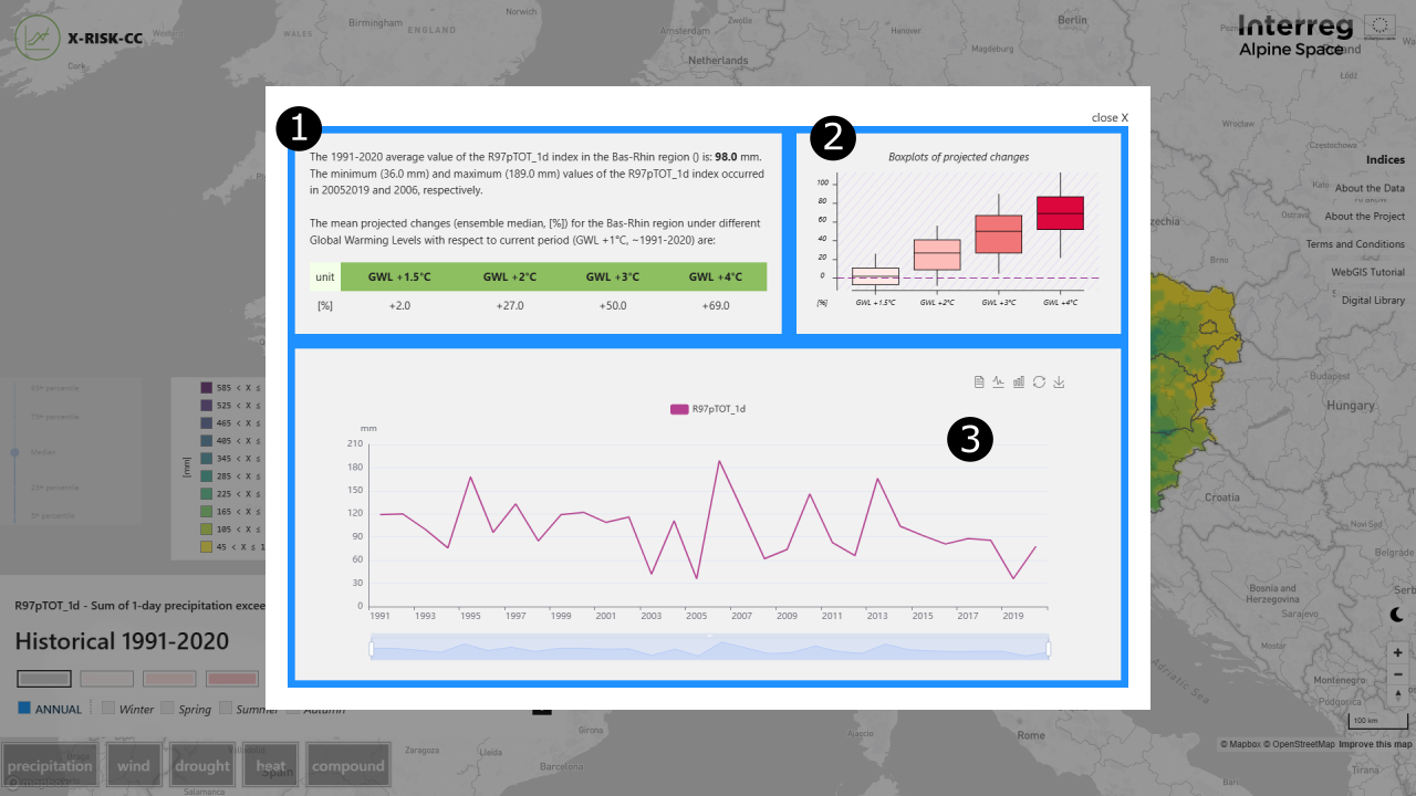
It reports specific index information for the selected region:

1. Top-left panel: The mean 1991-2020 value of the index and the years when the minimum and maximum values were recorded (as areal average). The table summarizing the mean projected changes with respect to 1991-2020 is reported.
2. Top-right panel: The boxplots with projected changes by the model ensemble over the GWLs. The horizontal bar is the median, the boxes extend over the interquartile range (25th – 75th percentile) and the whiskers between the 5th and 95th percentiles.
3. Bottom panel: the time series over the historical period (1991-2020) of the index with annual or seasonal aggregation. Through the slider below the plot, users can select and zoom in a specific period. Through the symbols in the top-right corner, the time series can be displayed in form of a table and the chart can be downloaded as a .png file1). For drought indices only, the time series report the monthly SPEI values (SPEI1 or SPEI3 depending on the index) over the period.